Fitter package

class controllers.fitter.Fit

Performs least square fitting, providing a couple of fit_functions

fit_functions

Name of fit functions as a list of strings. Possible values are:

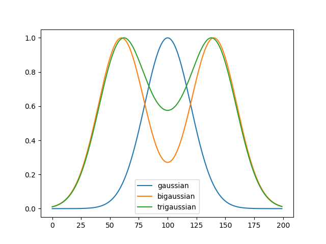
gaussian: \(y = h e^{ \frac{-(x - c)^ 2 } {2w^2}} + b\),

where h is the intensity, c the centre, b the offset, and w the variance of the distribution. Optimal for single profiles.

bigaussian: \(y = h_1 e^{ \frac{-(x - c_1)^ 2 } {2w_1^2}}+h_2 e^{ \frac{-(x - c_2)^ 2 } {2w_2^2}} + b\).

Optimal for profiles with dip.

trigaussian: \(y = h_1 e^{ \frac{-(x - c_1)^ 2 } {2w_1^2}}+ h_2 e^{ \frac{-(x - c_2)^ 2 } {2w_2^2}} + h_3 e^{ \frac{-(x - c_3)^ 2 } {2w_3^2}} + b\).

Optimal for profiles with dip and background.

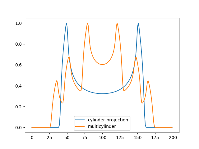
cylinder_projection: \(y = \Biggl \lbrace { h(\sqrt{r_2 ^2 - (x-c) ^ 2} - \sqrt{r_1 ^ 2 - (x-c) ^ 2}),\text{ if } \|x\| < r_2 \atop h(\sqrt{r_2 ^2 - (x-c) ^ 2}), \text{ if } \|x\| \geq r1, \|x\| < r_2 }\),

where r_1, r_2 denote the inner and outer cylinder radius. Describes the theoretical intensity profile for microtubule. The quality of the fit strongly depends on the initial estimation of the parameters, due to the nonlinearity of the cylinder function.

multi_cylinder_projection: \(y = cyl(i_1, c, 25e_x/2-2a, 25e_x/2-a) +\\ cyl(i_2, c, 42.5e_x/2, 42.5e_x/2+a) +\\ cyl(i_3, c, 25e_x/2+a,25e_x/2+2a) + b\),

this function assumes that a micrutubule sample was pre- and post labled under expansion microscopy (expansion factor \(e_x\)) the second cyl(cylinder_projection) compensates for pre labled fluorophores while the first and last cyl fit, post labled fluorophores considering a free orientation of the second antibody (antibody width a = 8.75).

Type:list(str)

Example

>>> fitter = fit_gaussian()
>>> X = np.linspace(0,199,200)

>>> gaussian = fit_gaussian.gaussian(X, 7.0, 20, 100, 0)
>>> gaussian = gaussian/gaussian.max()
>>> bigaussian = fitter.bigaussian(X, 6.0, 20, 140, 6.0, 20, 60, 0)
>>> bigaussian = bigaussian/bigaussian.max()
>>> trigaussian = fitter.trigaussian(X, 6.0, 20, 140, 6.0, 20, 60, 2.0, 20, 100, 0)
>>> trigaussian = trigaussian/trigaussian.max()
>>> plt.plot(gaussian, label="gaussian")
>>> plt.plot(bigaussian, label= "bigaussian")
>>> plt.plot(trigaussian, label="trigaussian")
>>> plt.legend(loc='best')
>>> plt.show()

>>> cylinder_proj = fit_gaussian.cylinder_projection(X, 25,100, 50, 60, 0,blur=1,)
>>> cylinder_proj = cylinder_proj/cylinder_proj.max()
>>> multicylinder = fitter.multi_cylinder_projection(X, 6, 6, 6, 100, 3, 0, blur= 1)
>>> multicylinder = multicylinder/multicylinder.max()
>>> plt.plot(cylinder_proj, label="cylinder-projection")
>>> plt.plot(multicylinder, label="multicylinder")
>>> plt.legend(loc='best')
>>> plt.show()

fit_data(data, center, nth_line=0, path=None, c=(1.0, 0.0, 0.0, 1.0), n_profiles=0)

Fit given data to functions in fit_functions. Creates a folder for each given function in “path”. A plot of input data the least square fit and the optimal parameters is saved as png.

Parameters:

• data (ndarray) –
• px_size (float [micro meter]) –
• sampling (int) –
• nth_line (int) – Extend path name with number on batch processing
• path (str) – Output data is saved in path
• c (tuple) – Defines the color of the data plot
• n_profiles (int) – Number of interpolated profiles. Is written as text in the plot.

class controllers.fitter.Hist

Plot data into a histogram and fit a right sided halfnorm to the histogram.

create_histogram(values, path=None, start=400, stop=1100)

Parameters:

• values (data to be fitted) –
• start (start for the plot) –
• stop (for the plot +100) –