Utility package

Utility package for image processing featuring funtcions like:

• Create gradient images
• Compute the orientation and position line resembling patterns in an image.
• Fit functions to a one dimensional dataset and save the plot in a given path

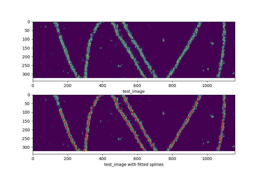
controllers.utility.compute_line_orientation(image, blur, min_len=10, spline=3, expansion=1, expansion2=1)

Compute the orientation and position of line resembling patterns in an image.

The image is convolved with a gaussian blur compensating for noise discontinuity or holes. A thresholding algorithm (1) converts the image from grayscale to binary. Using Lees algorithm (2) the expanded lines are reduced to one pixel width. The pixel coordinates from all still connected lines are retrieved and tested for continuity. Points of discontinuity are used as breakpoints and all following coordinates connected to a new line. Lines, shorter than the minimum required length are discarted. An univariate spline of degree 3 is fitted to each line. Note that shape and gradient of the line depend on the smoothing parameter. The rounded coordinates and their derivatives are returned in a table, together with the length of each line.

Parameters:

• image (ndarray) – Image containing line resembling patterns
• blur (int) – Amount of blur to apply to the image. Should be in the order of magnitude of the line width in pixel.
• min_len (int) – Minimal accepted line length
• smooth (float) – Positive smoothing factor used to choose the number of knots
• spline (int) – Degree of the smoothing spline. Must be <= 5. Default is 3, a cubic spline.

Returns:

• gradient_fitted_table (ndarray) – X, Y position of the splines. X, Y values of the spline gradient.
• shapes (ndarray) – Lengths of the lines written in gradient_fitted_table.

References

(1) Nobuyuki Otsu: A threshold selection method from grey level histograms. In: IEEE Transactions on Systems, Man, and Cybernetics. New York, 9.1979, S. 62–66. ISSN 1083-4419

(2) T.-C. Lee, R.L. Kashyap and C.-N. Chu, Building skeleton models via 3-D medial surface/axis thinning algorithms. Computer Vision, Graphics, and Image Processing, 56(6):462-478, 1994.

Example

>>> import matplotlib.pyplot as plt
>>> from src.controllers.utility import *
>>> import tifffile as tif
>>> import os
>>>
>>> with tif.TiffFile(os.path.dirname(os.getcwd()) + r"     est_data_microtub\Expansion dSTORM-Line Profile test.tif") as file:
>>>     image = file.asarray().astype(np.uint8)*40
>>>
>>> fig, axs = plt.subplots(2, 1, figsize=(9, 6), sharey=True)
>>> axs[0].imshow(image)
>>> axs[0].set_xlabel("test_image")
>>> axs[1].imshow(image)
>>> axs[1].set_xlabel("test_image with fitted splines")
>>> spline_table, shapes = compute_line_orientation(image, 20)
>>> spline_positions = spline_table[:,0:2]
>>> index = 0
>>> for i in range(len(shapes)):
>>>     axs[1].plot(spline_positions[index:index+shapes[i],1],spline_positions[index:index+shapes[i],0], c="r")
>>>     index += shapes[i]
>>> plt.show()

controllers.utility.create_floodfill_image(image)

Create a floodfill image applying a border with zeros around the image. This results in every boundary point, being a source point for the floodfill algorithm.

Parameters:image (ndarray) – 2D input image Returns:floodfill image – 2D binary output image Return type:ndarray

controllers.utility.create_gradient_image(image, blur, sobel=9)

Compute the Orientation of each pixel of a given image in rad

Parameters:

• image (ndarray) – Image data as numpy array in grayscale
• blur (int) – Blur image with a filter of blur kernel size
• sobel(optional) (int) – Kernel size of the applied sobel operators

Returns:

gradient_image – Array of the pixel orientation in a box of “sobel” size (unit = rad)

Return type:

ndarray

Example

>>> image = cv2.imread("path_to_file.png")
>>> gradient_image = create_gradient_image(image, 3)

controllers.utility.find_maximas(data, n=3)

Return the n biggest local maximas of a given 1d array.

Parameters:

• data (ndarray) – Input data
• n (int) – Number of local maximas to find

Returns:

values – Indices of local maximas.

Return type:

ndarray

controllers.utility.fit_data_to(func, x, data, expansion=1, chi_squared=False, center=None)

Fit data to given func using least square optimization. Compute and print chi2. Return the optimal parameters found for two gaussians.

Parameters:data (ndarray) – Given data (1d) Returns:optim2 – Optimal parameters Return type:tuple

controllers.utility.line_parameters(point, direction, width)

Parameters:

• point (tuple) – starting point for line
• direction (float) – direction of line

Returns:

result – Containing arrays with X and Y coordinates of line as well as start and endpoint

Return type:

dict

controllers.utility.order_points_to_line(points)

Determine the two nearest neighbors of each input point. Write the connectivity in a sparse matrix. Determine the order of the points.

Parameters:points (ndarray) – Sort input points (nx2) to a line Returns:points – Sorted output points Return type:ndarray